import arviz as az
import bambi as bmb
import matplotlib.pyplot as plt
import numpy as np
import pandas as pd
import pymc as pmGaussian Processes in 2D
This article demonstrates how to use Bambi with Gaussian Processes with 2 dimensional predictors. Bambi supports Gaussian Processes through the low-rank approximation known as Hilbert Space Gaussian Processes. For references see Hilbert Space Methods for Reduced-Rank Gaussian Process Regression and Practical Hilbert Space Approximate Bayesian Gaussian Processes for Probabilistic Programming.
If you prefer a video format, have a look at Introduction to Hilbert Space GPs in PyMC given by Bill Engels.
The goal of this notebook is to showcase Bambi’s support for Gaussian Processes on two-dimensional data using the HSGP approximation.
To achieve this, we begin by creating a matrix of coordinates that will serve as the locations where we measure the values of a continuous response variable.
x1 = np.linspace(0, 10, 12)
x2 = np.linspace(0, 10, 12)
xx, yy = np.meshgrid(x1, x2)
X = np.column_stack([xx.flatten(), yy.flatten()])
X.shape
(144, 2)Isotropic samples
In modeling multi-dimensional data with a Gaussian Process, we must choose between using an isotropic or an anisotropic Gaussian Process. An isotropic GP applies the same degree of smoothing to all predictors and is rotationally invariant. On the other hand, an anisotropic GP assigns different degrees of smoothing to each predictor and is not rotationally invariant.
Furthermore, as the hsgp() function allows for the creation of separate GP contribution terms for the levels of a categorical variable through its by argument, we also examine both single-group and multiple-group scenarios.
A single group
We create a covariance kernel using ExpQuad from the gp submodule in PyMC. Note that the lengthscale and amplitude for both dimensions are 2 and 1.2, respectively. Then, we simply use NumPy to get a random draw from the 144-dimensional multivariate normal distribution.
rng = np.random.default_rng(1234)

ell = 2
cov = 1.2 * pm.gp.cov.ExpQuad(2, ls=ell)
K = cov(X).eval()
mu = np.zeros(X.shape[0])
print(mu.shape, K.shape)

f = rng.multivariate_normal(mu, K)

fig, ax = plt.subplots()
ax.scatter(xx, yy, c=f, s=900, marker="s");
(144,) (144, 144)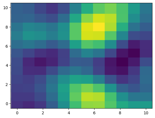
Since Bambi works with long-format data frames, we need to reshape our data before creating the data frame.
data = pd.DataFrame(
    {
        "x": np.tile(xx.flatten(), 1),
        "y": np.tile(yy.flatten(), 1),
        "outcome": f.flatten()
    }
)
Now, let’s construct the model. The only notable distinction from the one-dimensional case is that we provide two unnamed arguments to the hsgp() function, representing the predictors on each dimension.
prior_hsgp = {
    "sigma": bmb.Prior("Exponential", lam=3),
    "ell": bmb.Prior("InverseGamma", mu=2, sigma=0.2),
}
priors = {
    "hsgp(x, y, c=1.5, m=10)": prior_hsgp,
    "sigma": bmb.Prior("HalfNormal", sigma=2)
}
model = bmb.Model("outcome ~ 0 + hsgp(x, y, c=1.5, m=10)", data, priors=priors)
model.set_alias({"hsgp(x, y, c=1.5, m=10)": "hsgp"})
model
Formula: outcome ~ 0 + hsgp(x, y, c=1.5, m=10)
Family: gaussian
Link: mu = identity
Observations: 144
Priors:
target = mu
HSGP contributions
hsgp(x, y, c=1.5, m=10)
cov: ExpQuad
sigma ~ Exponential(lam: 3.0)
ell ~ InverseGamma(mu: 2.0, sigma: 0.2)
Auxiliary parameters
sigma ~ HalfNormal(sigma: 2.0)The parameters c and m of the HSGP aproximation are specific to each dimension, and can have different values for each. However, as we are passing scalars instead of sequences, Bambi will internally recycle them, causing the HSGP approximation to use the same values of c and m for both dimensions.
Let’s build the internal PyMC model and create a graph to have a visual representation of the relationships between the model parameters.
model.build()
model.graph()
And finally, we quickly fit the model and show a traceplot to explore the posterior and spot any issues with the sampler.
idata = model.fit(inference_method="nutpie", target_accept=0.9, num_chains=4)
print(idata.sample_stats.diverging.sum().item())
Sampler Progress
Total Chains: 4
Active Chains: 0
Finished Chains: 4
Sampling for now
Estimated Time to Completion: now
| Progress | Draws | Divergences | Step Size | Gradients/Draw |
|---|---|---|---|---|
| 2000 | 0 | 0.04 | 255 | |
| 2000 | 0 | 0.04 | 511 | |
| 2000 | 0 | 0.04 | 511 | |
| 2000 | 0 | 0.03 | 767 |
0az.plot_trace(
idata,
var_names=["hsgp_sigma", "hsgp_ell", "sigma"],
backend_kwargs={"layout": "constrained"}
);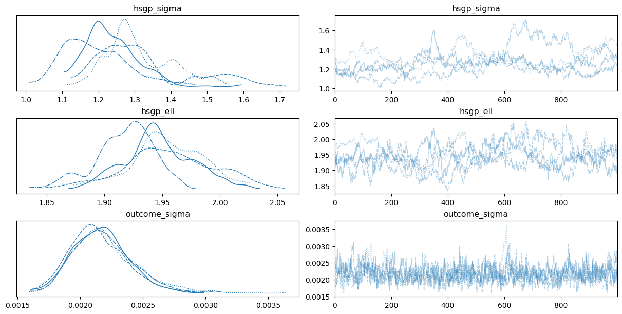
We don’t see any divergences. However, the autocorrelation in the chains for the covariance function parameters, along with the insufficient mixing, indicates that there may be an issue with the prior specification of the model.
Since the goal of the notebook is to simply show what features Bambi supports and how to use them, we won’t further investigate these issues. However, such posteriors shouldn’t be considered in any serious application.
From now on, the notebook will follow the same structure as the one already shown, which consists of
- Data simulation with some specific settings
- Creation of the Bambi model
- Building of the internal PyMC model and visualization of the graph
- Model fit and inspection of the traceplot
Multiple groups - same covariance function
In this scenario we have multiple groups that share the same covariance function.
rng = np.random.default_rng(123)

ell = 2
cov = 1.2 * pm.gp.cov.ExpQuad(2, ls=ell)
K = cov(X).eval()
mu = np.zeros(X.shape[0])

f = rng.multivariate_normal(mu, K, 3)

fig, axes = plt.subplots(1, 3, figsize=(12, 4))
for i, ax in enumerate(axes):
    ax.scatter(xx, yy, c=f[i], s=320, marker="s")
    ax.grid(False)
    ax.set_title(f"Group {i}")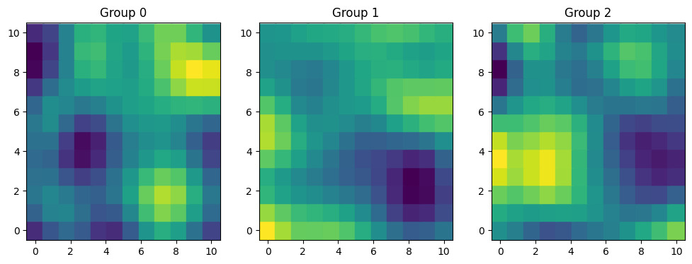
data = pd.DataFrame(
    {
        "x": np.tile(xx.flatten(), 3),
        "y": np.tile(yy.flatten(), 3),
        "group": np.repeat(list("ABC"), 12 * 12),
        "outcome": f.flatten()
    }
)
Notice we don’t modify anything substantial in the call to hsgp() for now.
prior_hsgp = {
    "sigma": bmb.Prior("Exponential", lam=3),
    "ell": bmb.Prior("InverseGamma", mu=2, sigma=0.2),
}
priors = {
    "hsgp(x, y, by=group, c=1.5, m=10)": prior_hsgp,
    "sigma": bmb.Prior("HalfNormal", sigma=2)
}
model = bmb.Model("outcome ~ 0 + hsgp(x, y, by=group, c=1.5, m=10)", data, priors=priors)
model.set_alias({"hsgp(x, y, by=group, c=1.5, m=10)": "hsgp"})
print(model)
model.build()
model.graph()
Formula: outcome ~ 0 + hsgp(x, y, by=group, c=1.5, m=10)
Family: gaussian
Link: mu = identity
Observations: 432
Priors:
target = mu
HSGP contributions
hsgp(x, y, by=group, c=1.5, m=10)
cov: ExpQuad
sigma ~ Exponential(lam: 3.0)
ell ~ InverseGamma(mu: 2.0, sigma: 0.2)
Auxiliary parameters
sigma ~ HalfNormal(sigma: 2.0)
idata = model.fit(inference_method="nutpie", target_accept=0.9, num_chains=4)
print(idata.sample_stats.diverging.sum().item())
Sampler Progress
Total Chains: 4
Active Chains: 0
Finished Chains: 4
Sampling for 17 seconds
Estimated Time to Completion: now
| Progress | Draws | Divergences | Step Size | Gradients/Draw |
|---|---|---|---|---|
| 2000 | 0 | 0.07 | 127 | |
| 2000 | 0 | 0.04 | 255 | |
| 2000 | 0 | 0.04 | 511 | |
| 2000 | 0 | 0.05 | 255 |
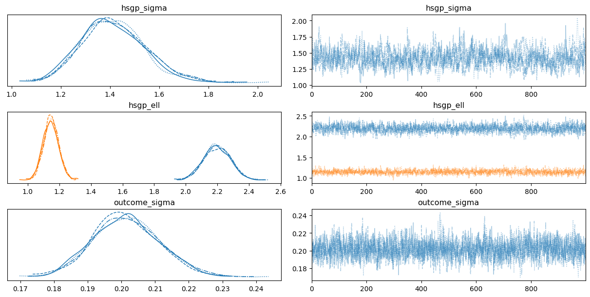
0az.plot_trace(
idata,
var_names=["hsgp_sigma", "hsgp_ell", "sigma"],
backend_kwargs={"layout": "constrained"}
);
While we have three groups, we only have one hsgp_sigma and one hsgp_ell for all groups. This is because, by default, the HSGP contributions by groups use the same instance of the covariance function.
Multiple groups - different covariance function
Again we have multiple groups. But this time, each group has specific values for the amplitude and the lengthscale.
rng = np.random.default_rng(12)

sigmas = [1.2, 1.5, 1.8]
ells = [1.5, 2, 3]

samples = []
for sigma, ell in zip(sigmas, ells):
    cov = sigma * pm.gp.cov.ExpQuad(2, ls=ell)
    K = cov(X).eval()
    mu = np.zeros(X.shape[0])
    samples.append(rng.multivariate_normal(mu, K))

f = np.stack(samples)
fig, axes = plt.subplots(1, 3, figsize=(12, 4))
for i, ax in enumerate(axes):
    ax.scatter(xx, yy, c=f[i], s=320, marker="s")
    ax.grid(False)
    ax.set_title(f"Group {i}")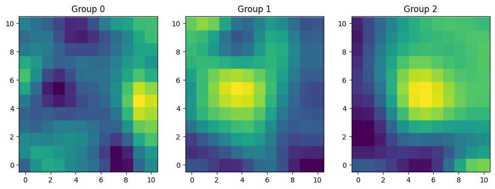
data = pd.DataFrame(
    {
        "x": np.tile(xx.flatten(), 3),
        "y": np.tile(yy.flatten(), 3),
        "group": np.repeat(list("ABC"), 12 * 12),
        "outcome": f.flatten()
    }
)
In situations like this, we can tell Bambi not to use the same covariance function for all the groups with share_cov=False and Bambi will create a separate instance for each group, resulting in group specific estimates of the amplitude and the lengthscale.
Notice, however, we’re still using the same kind of covariance function, which in this case is ExpQuad.
prior_hsgp = {
    "sigma": bmb.Prior("Exponential", lam=3),
    "ell": bmb.Prior("InverseGamma", mu=2, sigma=0.2),
}
priors = {
    "hsgp(x, y, by=group, c=1.5, m=10, share_cov=False)": prior_hsgp,
    "sigma": bmb.Prior("HalfNormal", sigma=2)
}
model = bmb.Model(
    "outcome ~ 0 + hsgp(x, y, by=group, c=1.5, m=10, share_cov=False)",
    data,
    priors=priors
)
model.set_alias({"hsgp(x, y, by=group, c=1.5, m=10, share_cov=False)": "hsgp"})
print(model)
model.build()
model.graph()
Formula: outcome ~ 0 + hsgp(x, y, by=group, c=1.5, m=10, share_cov=False)
Family: gaussian
Link: mu = identity
Observations: 432
Priors:
target = mu
HSGP contributions
hsgp(x, y, by=group, c=1.5, m=10, share_cov=False)
cov: ExpQuad
sigma ~ Exponential(lam: 3.0)
ell ~ InverseGamma(mu: 2.0, sigma: 0.2)
Auxiliary parameters
sigma ~ HalfNormal(sigma: 2.0)
See the all the HSGP related parameters gained the new dimension hsgp_by.
idata = model.fit(inference_method="nutpie", target_accept=0.9, num_chains=4)
print(idata.sample_stats.diverging.sum().item())
Sampler Progress
Total Chains: 4
Active Chains: 0
Finished Chains: 4
Sampling for 29 seconds
Estimated Time to Completion: now
| Progress | Draws | Divergences | Step Size | Gradients/Draw |
|---|---|---|---|---|
| 2000 | 0 | 0.06 | 511 | |
| 2000 | 0 | 0.06 | 767 | |
| 2000 | 0 | 0.06 | 511 | |
| 2000 | 0 | 0.06 | 511 |
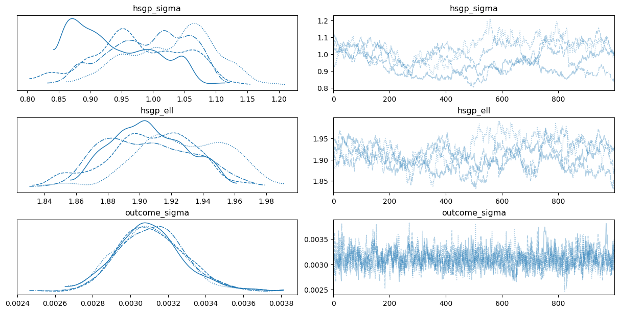
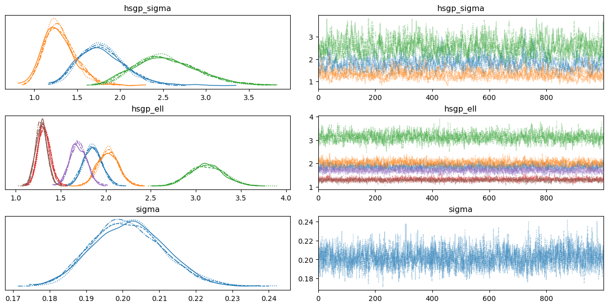
0az.plot_trace(
idata,
var_names=["hsgp_sigma", "hsgp_ell", "sigma"],
backend_kwargs={"layout": "constrained"}
);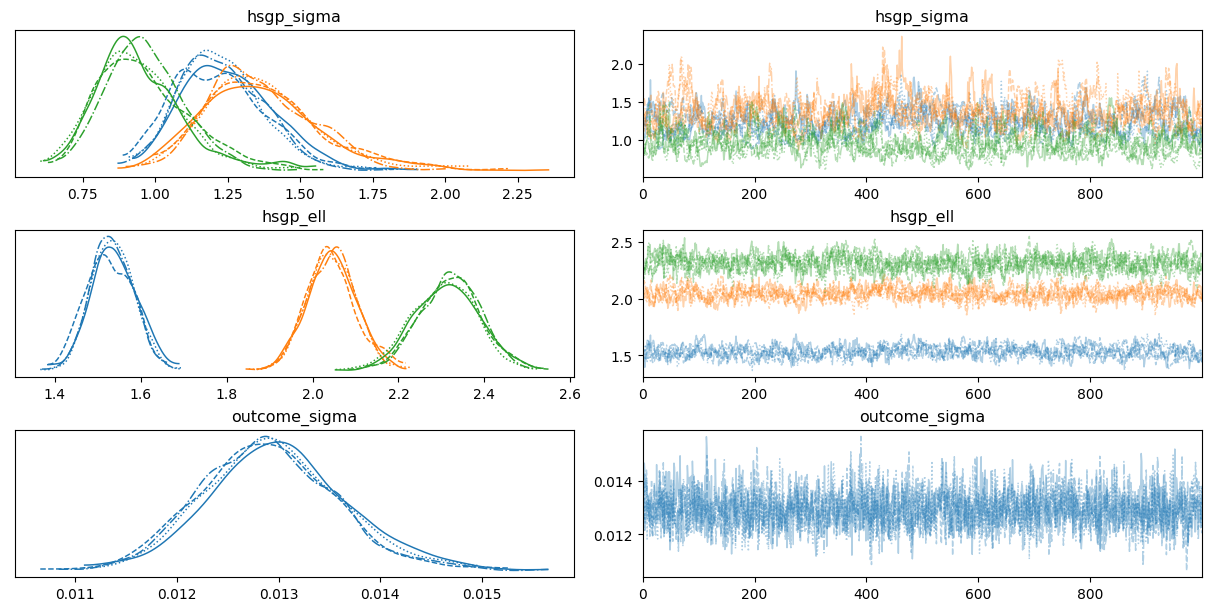
Unlike the previous case, now there are three hsgp_sigma and three hsgp_ell parameters, one per group. We can see them in different colors in the visualization.
Anisotropic samples
In this second part we repeat exactly the same that we did for the isotropic case. First, we start with a single group. Then, we continue with multiple groups that share the covariance function. And finally, multiple groups with different covariance functions. The main difference is that we use iso=False, which asks to use an anisotropic GP.
A single group
rng = np.random.default_rng(1234)

ell = [2, 0.9]
cov = 1.2 * pm.gp.cov.ExpQuad(2, ls=ell)
K = cov(X).eval()
mu = np.zeros(X.shape[0])

f = rng.multivariate_normal(mu, K)

fig, ax = plt.subplots(figsize = (4.5, 4.5))
ax.scatter(xx, yy, c=f, s=900, marker="s");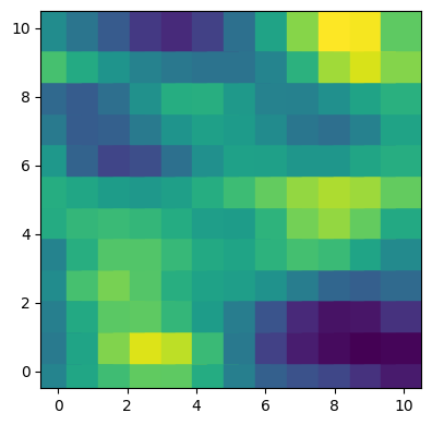
data = pd.DataFrame(
    {
        "x": np.tile(xx.flatten(), 1),
        "y": np.tile(yy.flatten(), 1),
        "outcome": f.flatten()
    }
)
prior_hsgp = {
"sigma": bmb.Prior("Exponential", lam=3),
"ell": bmb.Prior("InverseGamma", mu=2, sigma=0.2),
}
priors = {
"hsgp(x, y, c=1.5, m=10, iso=False)": prior_hsgp,
"sigma": bmb.Prior("HalfNormal", sigma=2)
}
model = bmb.Model("outcome ~ 0 + hsgp(x, y, c=1.5, m=10, iso=False)", data, priors=priors)
model.set_alias({"hsgp(x, y, c=1.5, m=10, iso=False)": "hsgp"})
print(model)
model.build()
model.graph() Formula: outcome ~ 0 + hsgp(x, y, c=1.5, m=10, iso=False)
Family: gaussian
Link: mu = identity
Observations: 144
Priors:
target = mu
HSGP contributions
hsgp(x, y, c=1.5, m=10, iso=False)
cov: ExpQuad
sigma ~ Exponential(lam: 3.0)
ell ~ InverseGamma(mu: 2.0, sigma: 0.2)
Auxiliary parameters
sigma ~ HalfNormal(sigma: 2.0)
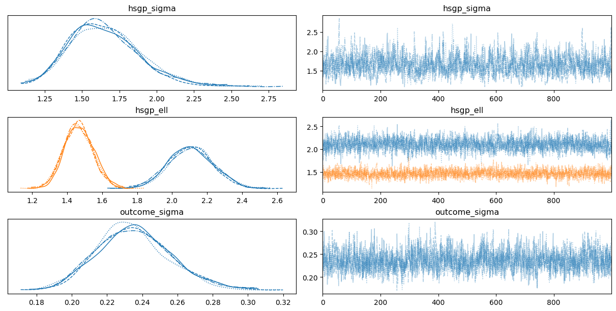
Although there is only one group in this case, the graph includes a hsgp_var dimension. This dimension represents the variables in the HSGP component, indicating that there is one lengthscale parameter per variable.
idata = model.fit(inference_method="nutpie", target_accept=0.9, num_chains=4)
print(idata.sample_stats.diverging.sum().item())
Sampler Progress
Total Chains: 4
Active Chains: 0
Finished Chains: 4
Sampling for now
Estimated Time to Completion: now
| Progress | Draws | Divergences | Step Size | Gradients/Draw |
|---|---|---|---|---|
| 2000 | 0 | 0.21 | 63 | |
| 2000 | 0 | 0.20 | 31 | |
| 2000 | 0 | 0.20 | 31 | |
| 2000 | 0 | 0.21 | 31 |
0az.plot_trace(
idata,
var_names=["hsgp_sigma", "hsgp_ell", "sigma"],
backend_kwargs={"layout": "constrained"}
);
Multiple groups - same covariance function
rng = np.random.default_rng(123)

ell = [2, 0.9]
cov = 1.2 * pm.gp.cov.ExpQuad(2, ls=ell)
K = cov(X).eval()
mu = np.zeros(X.shape[0])

f = rng.multivariate_normal(mu, K, 3)

fig, axes = plt.subplots(1, 3, figsize=(12, 4))
for i, ax in enumerate(axes):
    ax.scatter(xx, yy, c=f[i], s=320, marker="s")
    ax.grid(False)
    ax.set_title(f"Group {i}")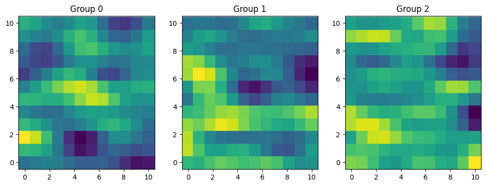
data = pd.DataFrame(
    {
        "x": np.tile(xx.flatten(), 3),
        "y": np.tile(yy.flatten(), 3),
        "group": np.repeat(list("ABC"), 12 * 12),
        "outcome": f.flatten()
    }
)
prior_hsgp = {
"sigma": bmb.Prior("Exponential", lam=3),
"ell": bmb.Prior("InverseGamma", mu=2, sigma=0.2),
}
priors = {
"hsgp(x, y, by=group, c=1.5, m=10, iso=False)": prior_hsgp,
"sigma": bmb.Prior("HalfNormal", sigma=2)
}
model = bmb.Model("outcome ~ 0 + hsgp(x, y, by=group, c=1.5, m=10, iso=False)", data, priors=priors)
model.set_alias({"hsgp(x, y, by=group, c=1.5, m=10, iso=False)": "hsgp"})
print(model)
model.build()
model.graph() Formula: outcome ~ 0 + hsgp(x, y, by=group, c=1.5, m=10, iso=False)
Family: gaussian
Link: mu = identity
Observations: 432
Priors:
target = mu
HSGP contributions
hsgp(x, y, by=group, c=1.5, m=10, iso=False)
cov: ExpQuad
sigma ~ Exponential(lam: 3.0)
ell ~ InverseGamma(mu: 2.0, sigma: 0.2)
Auxiliary parameters
sigma ~ HalfNormal(sigma: 2.0)
idata = model.fit(inference_method="nutpie", target_accept=0.9, num_chains=4)
print(idata.sample_stats.diverging.sum().item())
Sampler Progress
Total Chains: 4
Active Chains: 0
Finished Chains: 4
Sampling for now
Estimated Time to Completion: now
| Progress | Draws | Divergences | Step Size | Gradients/Draw |
|---|---|---|---|---|
| 2000 | 0 | 0.17 | 31 | |
| 2000 | 0 | 0.17 | 63 | |
| 2000 | 0 | 0.17 | 63 | |
| 2000 | 0 | 0.17 | 31 |
0az.plot_trace(
idata,
var_names=["hsgp_sigma", "hsgp_ell", "sigma"],
backend_kwargs={"layout": "constrained"}
);
Multiple groups - different covariance function
rng = np.random.default_rng(12)

sigmas = [1.2, 1.5, 1.8]
ells = [[1.5, 0.8], [2, 1.5], [3, 1]]

samples = []
for sigma, ell in zip(sigmas, ells):
    cov = sigma * pm.gp.cov.ExpQuad(2, ls=ell)
    K = cov(X).eval()
    mu = np.zeros(X.shape[0])
    samples.append(rng.multivariate_normal(mu, K))

f = np.stack(samples)
fig, axes = plt.subplots(1, 3, figsize=(12, 4))
for i, ax in enumerate(axes):
    ax.scatter(xx, yy, c=f[i], s=320, marker="s")
    ax.grid(False)
    ax.set_title(f"Group {i}")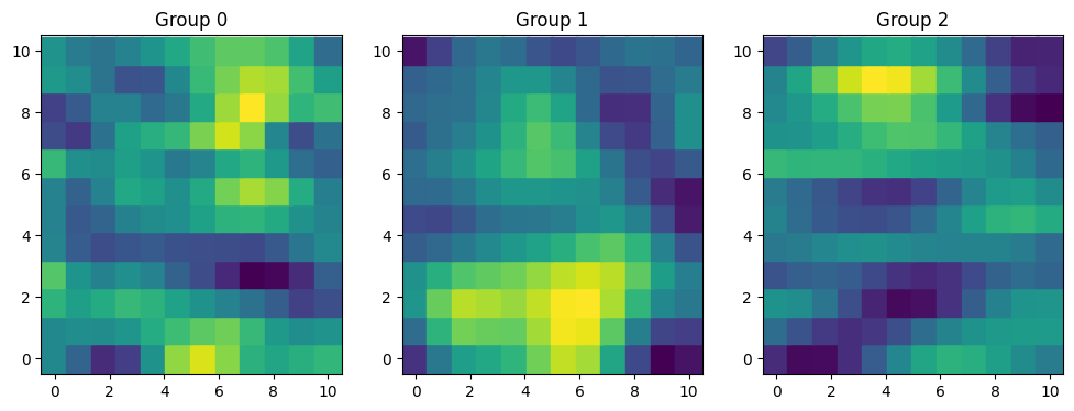
data = pd.DataFrame(
    {
        "x": np.tile(xx.flatten(), 3),
        "y": np.tile(yy.flatten(), 3),
        "group": np.repeat(list("ABC"), 12 * 12),
        "outcome": f.flatten()
    }
)
prior_hsgp = {
"sigma": bmb.Prior("Exponential", lam=3),
"ell": bmb.Prior("InverseGamma", mu=2, sigma=0.2),
}
priors = {
"hsgp(x, y, by=group, c=1.5, m=10, iso=False, share_cov=False)": prior_hsgp,
"sigma": bmb.Prior("HalfNormal", sigma=2)
}
model = bmb.Model(
"outcome ~ 0 + hsgp(x, y, by=group, c=1.5, m=10, iso=False, share_cov=False)",
data,
priors=priors
)
model.set_alias({"hsgp(x, y, by=group, c=1.5, m=10, iso=False, share_cov=False)": "hsgp"})
print(model)
model.build()
model.graph() Formula: outcome ~ 0 + hsgp(x, y, by=group, c=1.5, m=10, iso=False, share_cov=False)
Family: gaussian
Link: mu = identity
Observations: 432
Priors:
target = mu
HSGP contributions
hsgp(x, y, by=group, c=1.5, m=10, iso=False, share_cov=False)
cov: ExpQuad
sigma ~ Exponential(lam: 3.0)
ell ~ InverseGamma(mu: 2.0, sigma: 0.2)
Auxiliary parameters
sigma ~ HalfNormal(sigma: 2.0)
idata = model.fit(inference_method="nutpie", target_accept=0.9, num_chains=4)
print(idata.sample_stats.diverging.sum().item())
Sampler Progress
Total Chains: 4
Active Chains: 0
Finished Chains: 4
Sampling for now
Estimated Time to Completion: now
| Progress | Draws | Divergences | Step Size | Gradients/Draw |
|---|---|---|---|---|
| 2000 | 0 | 0.15 | 63 | |
| 2000 | 0 | 0.15 | 31 | |
| 2000 | 0 | 0.15 | 31 | |
| 2000 | 0 | 0.15 | 31 |
0az.plot_trace(
idata,
var_names=["hsgp_sigma", "hsgp_ell", "sigma"],
backend_kwargs={"layout": "constrained"}
);
A more complex example: Poisson likelihood with group-specific effects
For this final demonstration we’re going to use a simulated dataset where the outcome is a count variable. For the predictors, we have the location in terms of the latitude and longitude, as well as other variables such as the year of the measurement, the site where the measure was made, and one continuous predictor.
data = pd.read_csv("data/poisson_data.csv")
data["Year"] = pd.Categorical(data["Year"])
print(data.shape)
data.head()
(100, 6)| Year | Count | Site | Lat | Lon | X1 | |
|---|---|---|---|---|---|---|
| 0 | 2015 | 4 | Site1 | 47.559880 | 7.216754 | 3.316140 |
| 1 | 2016 | 0 | Site1 | 47.257079 | 7.135390 | 2.249612 |
| 2 | 2015 | 0 | Site1 | 47.061967 | 7.804383 | 2.835283 |
| 3 | 2016 | 0 | Site1 | 47.385533 | 7.433145 | 2.776692 |
| 4 | 2015 | 1 | Site1 | 47.034987 | 7.434643 | 2.295769 |
We can visualize the outcome variable by location and year.
fig, axes = plt.subplots(1, 2, figsize=(12, 4))
for i, (ax, year) in enumerate(zip(axes, [2015, 2016])):
    mask = data["Year"] == year
    x = data.loc[mask, "Lat"]
    y = data.loc[mask, "Lon"]
    count = data.loc[mask, "Count"]
    ax.scatter(x, y, c=count, s=30, marker="s")
    ax.set_title(f"Year {year}")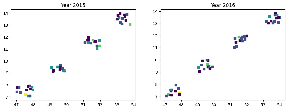
There’s not much we can conclude from here but it’s not a problem. The most relevant part of the example is not the data itself, but how to use Bambi to include GP components in a complex model.
It’s very easy to create a model that uses both regular common and group-specific predictors as well as a GP contribution term. We just add them to the model formula, treat hsgp() as any other call, and that’s it!
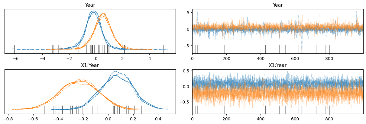
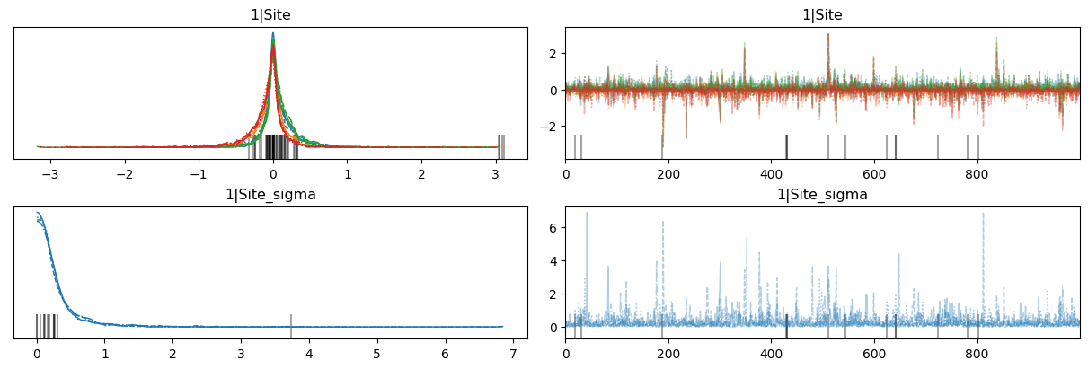
Below we have common effects for the Year, the interaction between X1 and Year, and group-specific intercepts by Site. Finally, we add hsgp() as any other call.
formula = "Count ~ 0 + Year + X1:Year + (1|Site) + hsgp(Lon, Lat, by=Year, m=5, c=1.5)"
model = bmb.Model(formula, data, family="poisson")
model
Formula: Count ~ 0 + Year + X1:Year + (1|Site) + hsgp(Lon, Lat, by=Year, m=5, c=1.5)
Family: poisson
Link: mu = log
Observations: 100
Priors:
target = mu
Common-level effects
Year ~ Normal(mu: [0. 0.], sigma: [5. 5.])
X1:Year ~ Normal(mu: [0. 0.], sigma: [1.5693 1.4766])
Group-level effects
1|Site ~ Normal(mu: 0.0, sigma: HalfNormal(sigma: 5.3683))
HSGP contributions
hsgp(Lon, Lat, by=Year, m=5, c=1.5)
cov: ExpQuad
sigma ~ Exponential(lam: 1.0)
ell ~ InverseGamma(alpha: 3.0, beta: 2.0)Let’s use an alias to make the graph representation more readable.
model.set_alias({"hsgp(Lon, Lat, by=Year, m=5, c=1.5)": "gp"})
model.build()
model.graph()
And finally, let’s fit the model.
idata = model.fit(inference_method="nutpie", target_accept=0.99, num_chains=4)
print(idata.sample_stats.diverging.sum().item())
Sampler Progress
Total Chains: 4
Active Chains: 0
Finished Chains: 4
Sampling for now
Estimated Time to Completion: now
| Progress | Draws | Divergences | Step Size | Gradients/Draw |
|---|---|---|---|---|
| 2000 | 0 | 0.07 | 63 | |
| 2000 | 1 | 0.06 | 63 | |
| 2000 | 2 | 0.06 | 63 | |
| 2000 | 4 | 0.08 | 63 |
7az.plot_trace(
idata,
var_names=["gp_sigma", "gp_ell", "gp_weights"],
backend_kwargs={"layout": "constrained"}
);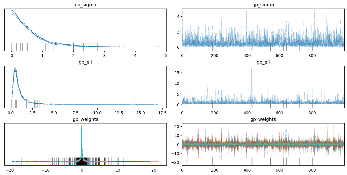
Notice the posteriors for the gp_weights are all centered at zero. This is a symptom of the absence of any spatial effect.
az.plot_trace(
    idata,
    var_names=["Year", "X1:Year"],
    backend_kwargs={"layout": "constrained"}
);
az.plot_trace(
    idata,
    var_names=["1|Site", "1|Site_sigma"],
    backend_kwargs={"layout": "constrained"}
);
%load_ext watermark
%watermark -n -u -v -iv -w
Last updated: Tue Dec 16 2025
Python implementation: CPython
Python version : 3.13.9
IPython version : 9.6.0
arviz : 0.22.0
matplotlib: 3.10.7
bambi : 0.15.1.dev47+g707bbd9e5.d20251216
numpy : 2.3.3
pandas : 2.3.3
pymc : 5.26.1
Watermark: 2.5.0