Bambi – how_bambi

Basic building blocks

Linear predictor

Bambi builds linear predictors of the form

\[ \pmb{\eta} = \mathbf{X}\pmb{\beta} + \mathbf{Z}\pmb{u} \]

The linear predictor is the sum of two kinds of contributions

\(\mathbf{X}\pmb{\beta}\) is the common (fixed) effects contribution
\(\mathbf{Z}\pmb{u}\) is the group-specific (random) effects contribution

Both contributions obey the same rule: A dot product between a data object and a parameter object.

Design matrix

The following objects are design matrices

\[ \begin{array}{c} \underset{n\times p}{\mathbf{X}} & \underset{n\times j}{\mathbf{Z}} \end{array} \]

\(\mathbf{X}\) is the design matrix for the common (fixed) effects part
\(\mathbf{Z}\) is the design matrix for the group-specific (random) effects part

Parameter vector

The following objects are parameter vectors

\[ \begin{array}{c} \underset{p\times 1}{\pmb{\beta}} & \underset{j\times 1}{\pmb{u}} \end{array} \]

\(\pmb{\beta}\) is a vector of parameters/coefficients for the common (fixed) effects part
\(\pmb{u}\) is a vector of parameters/coefficients for the group-specific (random) effects part

As result, the linear predictor \(\pmb{\eta}\) is of shape \(n \times 1\).

A fundamental question: How do we use linear predictors in modeling?

Linear predictors (or a function of them) describe the functional relationship between one or more parameters of the response distribution and the predictors.

Example: Linear regression

A classical linear regression model is a special case where there is no group-specific contribution and a linear predictor is mapped to the mean parameter of the response distribution.

\[ \begin{aligned} \pmb{\mu} &= \pmb{\eta} = \mathbf{X}\pmb{\beta} \\ \pmb{\beta} &\sim \text{Distribution} \\ \sigma &\sim \text{Distribution} \\ Y_i &\sim \text{Normal}(\eta_i, \sigma) \end{aligned} \]

Link functions

Link functions turn linear models in generalized linear models. A link function, \(g\), is a function that maps a parameter of the response distribution to the linear predictor. When people talk about generalized linear models, they mean there’s a link function mapping the mean of the response distribution to the linear predictor. But as we will see later, Bambi allows to use linear predictors and link functions to model any parameter of the response distribution – these are known as distributional models or generalized linear models for location, scale, and shape.

\[ g(\pmb{\mu}) = \pmb{\eta} = \mathbf{X}\pmb{\beta} \]

where \(g\) is the link function. It must be differentiable, monotonic, and invertible. For example, the logit function is useful when the mean parameter is bounded in the \((0, 1)\) domain.

\[ \begin{aligned} g(\pmb{\mu}) &= \text{logit}(\pmb{\mu}) = \log \left(\frac{\pmb{\mu}}{1 - \pmb{\mu}}\right) = \pmb{\eta} = \mathbf{X}\pmb{\beta} \\ \pmb{\mu} = g^{-1}(\pmb{\eta}) &= \text{logistic}(\pmb{\eta}) = \frac{1}{1 + \exp (-\pmb{\eta})} = \frac{1}{1 + \exp (-\mathbf{X}\pmb{\beta})} \end{aligned} \]

Example: Logistic regression

\[ \begin{aligned} g(\pmb{\mu}) &= \mathbf{X}\pmb{\beta} \\ \pmb{\beta} &\sim \text{Distribution} \\ Y_i &\sim \text{Bernoulli}(\mu = g^{-1}(\mathbf{X}\pmb{\beta} )_i) \end{aligned} \]

where \(g = \text{logit}\) and \(g^{-1} = \text{logistic}\) also known as \(\text{expit}\).

Generalized linear models for location, scale, and shape

This is an extension to generalized linear models. In a generalized linear model a linear predictor and a link function are used to explain the relationship between the mean (location) of the response distribution and the predictors. In this type of models we are able to use linear predictors and link functions to represent the relationship between any parameter of the response distribution and the predictors.

\[ \begin{aligned} g_1(\pmb{\theta}_1) &= \mathbf{X}_1\pmb{\beta}_1 + \mathbf{Z}_1\pmb{u}_1 \\ g_2(\pmb{\theta}_2) &= \mathbf{X}_2\pmb{\beta}_2 + \mathbf{Z}_2\pmb{u}_2 \\ &\phantom{b=\,} \vdots \\ g_k(\pmb{\theta}_k) &= \mathbf{X}_k\pmb{\beta}_k + \mathbf{Z}_k\pmb{u}_k \\ Y_i &\sim \text{Distribution}(\theta_{1i}, \theta_{2i}, \dots, \theta_{ki}) \end{aligned} \]

Example: Heteroskedastic linear regression

\[ \begin{aligned} g_1(\pmb{\mu}) &= \mathbf{X}_1\pmb{\beta}_1 \\ g_2(\pmb{\sigma}) &= \mathbf{X}_2\pmb{\beta}_2 \\ \pmb{\beta}_1 &\sim \text{Distribution} \\ \pmb{\beta}_2 &\sim \text{Distribution} \\ Y_i &\sim \text{Normal}(\mu_i, \sigma_i) \end{aligned} \]

Where

\(g_1\) is the identity function
\(g_2\) is a function that maps \(\mathbb{R}\to\mathbb{R}^+\).
- Usually \(g_2 = \log\)
- \(\pmb{\sigma} = \exp(\mathbf{X}_2\pmb{\beta}_2)\).

What can be included in a design matrix

A design matrix is… a matrix. As such, it’s filled up with numbers. However, it does not mean it cannot encode non-numerical variables. In a design matrix we can encode the following

Numerical predictors
Interaction effects
Transformations of numerical predictors that don’t depend on model parameters
- Powers
- Centering
- Standardization
- Basis functions
  - Bambi currently supports basis splines
- And anything you can imagine as well as it does not involve model parameters
Categorical predictors
- Categorical variables are encoded into their own design matrices
- The most popular approach is to create binary “dummy” variables. One per level of the categorical variable.
- But doing it haphazardly will result in non-identifiabilities quite soon.
- Encodings to the rescue
  - One can apply different restrictions or contrast matrices to overcome this problem. They usually imply different interpretations of the regression coefficients.
  - Treatment encoding: Sets one level to zero
  - Zero-sum encoding: Sets one level to the opposite of the sum of the other levels
  - Backward differences
  - Orthogonal polynomials
  - Helmert contrasts
  - …

These all can be expressed as a single set of columns of a design matrix that are matched with a subset of the parameter vector of the same length

Who takes care of each step?

Data matrices are built by formulae.
- Data matrices are not dependent on parameter values in any form.
Bambi consumes and manipulates them to create model terms, which shape the parameter vector.
- The parameter vector is not influenced by the values in the data matrix.

Going back to planet Earth…

Example

import arviz as az
import bambi as bmb
import matplotlib.pyplot as plt
import numpy as np
import pandas as pd

az.style.use("arviz-darkgrid")

data = bmb.load_data("sleepstudy")

def plot_data(data):
    fig, axes = plt.subplots(2, 9, figsize=(16, 7.5), sharey=True, sharex=True, dpi=300, constrained_layout=False)
    fig.subplots_adjust(left=0.075, right=0.975, bottom=0.075, top=0.925, wspace=0.03)

    axes_flat = axes.ravel()

    for i, subject in enumerate(data["Subject"].unique()):
        ax = axes_flat[i]
        idx = data.index[data["Subject"] == subject].tolist()
        days = data.loc[idx, "Days"].to_numpy()
        reaction = data.loc[idx, "Reaction"].to_numpy()

        # Plot observed data points
        ax.scatter(days, reaction, color="C0", ec="black", alpha=0.7)

        # Add a title
        ax.set_title(f"Subject: {subject}", fontsize=14)

    ax.xaxis.set_ticks([0, 2, 4, 6, 8])
    fig.text(0.5, 0.02, "Days", fontsize=14)
    fig.text(0.03, 0.5, "Reaction time (ms)", rotation=90, fontsize=14, va="center")

    return axes

plot_data(data);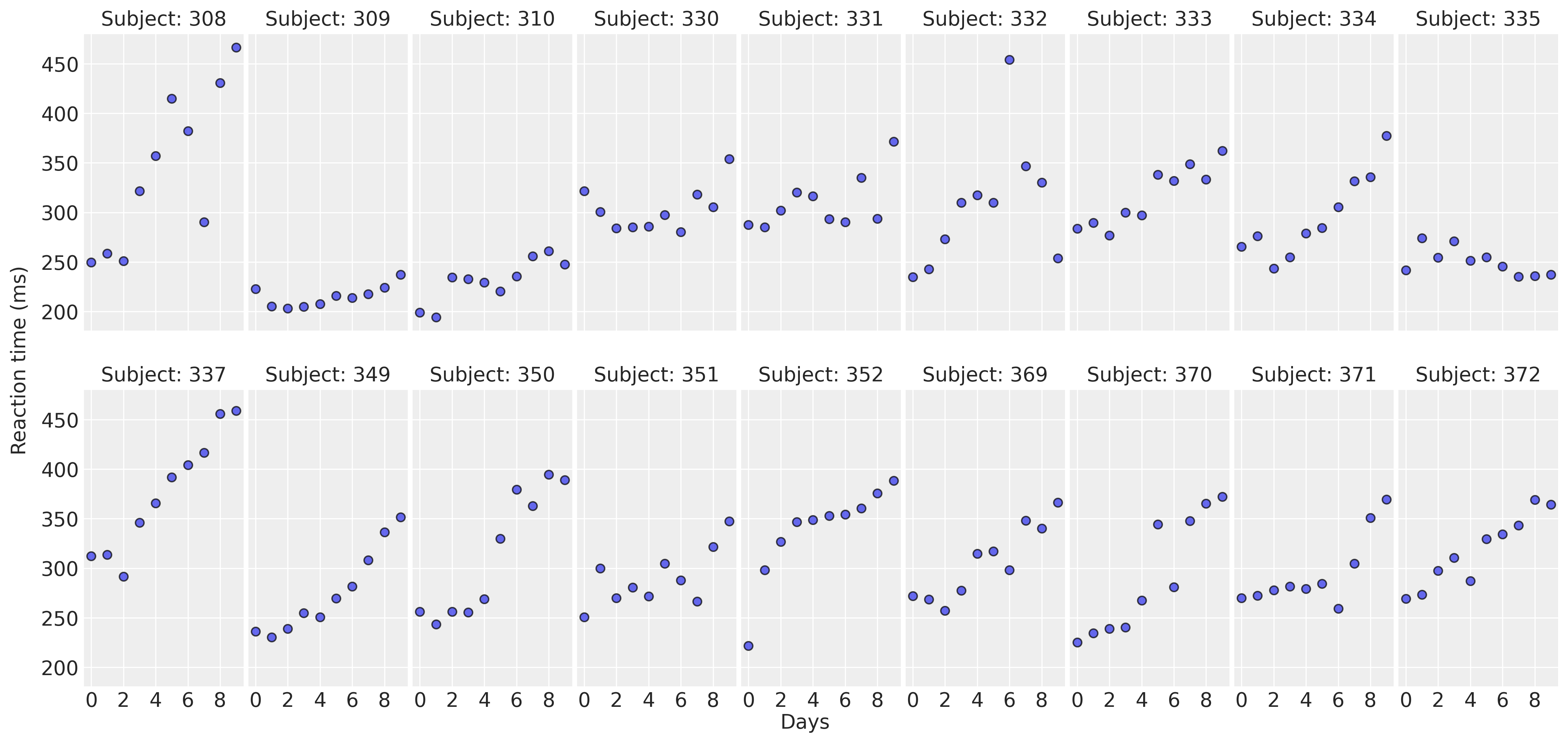

The model

\[ \begin{aligned} \mu_i & = \beta_0 + \beta_1 \text{Days}_i + u_{0i} + u_{1i}\text{Days}_i \\ \beta_0 & \sim \text{Normal} \\ \beta_1 & \sim \text{Normal} \\ u_{0i} & \sim \text{Normal}(0, \sigma_{u_0}) \\ u_{1i} & \sim \text{Normal}(0, \sigma_{u_1}) \\ \sigma_{u_0} & \sim \text{HalfNormal} \\ \sigma_{u_1} & \sim \text{HalfNormal} \\ \sigma & \sim \text{HalfStudentT} \\ \text{Reaction}_i & \sim \text{Normal}(\mu_i, \sigma) \end{aligned} \]

Written in a slightly different way (and omitting some priors)…

\[ \begin{aligned} \mu_i & = \text{Intercept}_i + \text{Slope}_i \text{Days}_i \\ \text{Intercept}_i & = \beta_0 + u_{0i} \\ \text{Slope}_i & = \beta_1 + u_{1i} \\ \sigma & \sim \text{HalfStudentT} \\ \text{Reaction}_i & \sim \text{Normal}(\mu_i, \sigma) \\ \end{aligned} \]

We can see both the intercept and the slope are made of a “common” component and a “subject-specific” deflection.

Under the general representation written above…

\[ \begin{aligned} \pmb{\mu} &= \mathbf{X}\pmb{\beta} + \mathbf{Z}\pmb{u} \\ \pmb{\beta} &\sim \text{Normal} \\ \pmb{u} &\sim \text{Normal}(0, \text{diag}(\sigma_{\pmb{u}})) \\ \sigma &\sim \text{HalfStudenT} \\ \sigma_{\pmb{u}} &\sim \text{HalfNormal} \\ Y_i &\sim \text{Normal}(\mu_i, \sigma) \end{aligned} \]

model = bmb.Model("Reaction ~ 1 + Days + (1 + Days | Subject)", data, categorical="Subject")
model

       Formula: Reaction ~ 1 + Days + (1 + Days | Subject)
        Family: gaussian
          Link: mu = identity
  Observations: 180
        Priors: 
    target = mu
        Common-level effects
            Intercept ~ Normal(mu: 298.5079, sigma: 261.0092)
            Days ~ Normal(mu: 0.0, sigma: 48.8915)
        
        Group-level effects
            1|Subject ~ Normal(mu: 0.0, sigma: HalfNormal(sigma: 261.0092))
            Days|Subject ~ Normal(mu: 0.0, sigma: HalfNormal(sigma: 48.8915))
        
        Auxiliary parameters
            Reaction_sigma ~ HalfStudentT(nu: 4.0, sigma: 56.1721)

model.build()
model.graph()

dm = model.response_component.design
dm

DesignMatrices

                  (rows, cols)
Response:               (180,)
Common:               (180, 2)
Group-specific:      (180, 36)

Use .reponse, .common, or .group to access the different members.

print(dm.response, "\n")
print(np.array(dm.response)[:5])

ResponseMatrix  
  name: Reaction
  kind: numeric
  shape: (180,)

To access the actual design matrix do 'np.array(this_obj)' 

[249.56   258.7047 250.8006 321.4398 356.8519]

print(dm.common, "\n")
print(np.array(dm.common)[:5])

CommonEffectsMatrix with shape (180, 2)
Terms:  
  Intercept  
    kind: intercept
    column: 0
  Days  
    kind: numeric
    column: 1

To access the actual design matrix do 'np.array(this_obj)' 

[[1 0]
 [1 1]
 [1 2]
 [1 3]
 [1 4]]

print(dm.group, "\n")
print(np.array(dm.group)[:14])

GroupEffectsMatrix with shape (180, 36)
Terms:  
  1|Subject  
    kind: intercept
    groups: ['308', '309', '310', '330', '331', '332', '333', '334', '335', '337', '349', '350',
      '351', '352', '369', '370', '371', '372']
    columns: 0:18
  Days|Subject  
    kind: numeric
    groups: ['308', '309', '310', '330', '331', '332', '333', '334', '335', '337', '349', '350',
      '351', '352', '369', '370', '371', '372']
    columns: 18:36

To access the actual design matrix do 'np.array(this_obj)' 

[[1 0 0 0 0 0 0 0 0 0 0 0 0 0 0 0 0 0 0 0 0 0 0 0 0 0 0 0 0 0 0 0 0 0 0 0]
 [1 0 0 0 0 0 0 0 0 0 0 0 0 0 0 0 0 0 1 0 0 0 0 0 0 0 0 0 0 0 0 0 0 0 0 0]
 [1 0 0 0 0 0 0 0 0 0 0 0 0 0 0 0 0 0 2 0 0 0 0 0 0 0 0 0 0 0 0 0 0 0 0 0]
 [1 0 0 0 0 0 0 0 0 0 0 0 0 0 0 0 0 0 3 0 0 0 0 0 0 0 0 0 0 0 0 0 0 0 0 0]
 [1 0 0 0 0 0 0 0 0 0 0 0 0 0 0 0 0 0 4 0 0 0 0 0 0 0 0 0 0 0 0 0 0 0 0 0]
 [1 0 0 0 0 0 0 0 0 0 0 0 0 0 0 0 0 0 5 0 0 0 0 0 0 0 0 0 0 0 0 0 0 0 0 0]
 [1 0 0 0 0 0 0 0 0 0 0 0 0 0 0 0 0 0 6 0 0 0 0 0 0 0 0 0 0 0 0 0 0 0 0 0]
 [1 0 0 0 0 0 0 0 0 0 0 0 0 0 0 0 0 0 7 0 0 0 0 0 0 0 0 0 0 0 0 0 0 0 0 0]
 [1 0 0 0 0 0 0 0 0 0 0 0 0 0 0 0 0 0 8 0 0 0 0 0 0 0 0 0 0 0 0 0 0 0 0 0]
 [1 0 0 0 0 0 0 0 0 0 0 0 0 0 0 0 0 0 9 0 0 0 0 0 0 0 0 0 0 0 0 0 0 0 0 0]
 [0 1 0 0 0 0 0 0 0 0 0 0 0 0 0 0 0 0 0 0 0 0 0 0 0 0 0 0 0 0 0 0 0 0 0 0]
 [0 1 0 0 0 0 0 0 0 0 0 0 0 0 0 0 0 0 0 1 0 0 0 0 0 0 0 0 0 0 0 0 0 0 0 0]
 [0 1 0 0 0 0 0 0 0 0 0 0 0 0 0 0 0 0 0 2 0 0 0 0 0 0 0 0 0 0 0 0 0 0 0 0]
 [0 1 0 0 0 0 0 0 0 0 0 0 0 0 0 0 0 0 0 3 0 0 0 0 0 0 0 0 0 0 0 0 0 0 0 0]]

model.response_component.intercept_term

CommonTerm(  
  name: Intercept,
  prior: Normal(mu: 298.5079, sigma: 261.0092),
  shape: (180,),
  categorical: False
)

model.response_component.common_terms

{'Days': CommonTerm(  
   name: Days,
   prior: Normal(mu: 0.0, sigma: 48.8915),
   shape: (180,),
   categorical: False
 )}

model.response_component.group_specific_terms

{'1|Subject': GroupSpecificTerm(  
   name: 1|Subject,
   prior: Normal(mu: 0.0, sigma: HalfNormal(sigma: 261.0092)),
   shape: (180, 18),
   categorical: False,
   groups: ['308', '309', '310', '330', '331', '332', '333', '334', '335', '337', '349', '350', '351', '352', '369', '370', '371', '372']
 ),
 'Days|Subject': GroupSpecificTerm(  
   name: Days|Subject,
   prior: Normal(mu: 0.0, sigma: HalfNormal(sigma: 48.8915)),
   shape: (180, 18),
   categorical: False,
   groups: ['308', '309', '310', '330', '331', '332', '333', '334', '335', '337', '349', '350', '351', '352', '369', '370', '371', '372']
 )}

Terms not only exist in the Bambi world. There are three (!!) types of terms being created.

Formulae has its terms
- Agnostic information design matrix information
Bambi has its terms
- Contains both the information given by formulae and metadata relevant to Bambi (priors)
The backend has its terms
- Accept a Bambi term and knows how to “compile” itself to that backend.
- E.g. the PyMC backend terms know how to write one or more PyMC distributions out of a Bambi term.

Could we have multiple backends? In principle yes. But there’s one aspect which is convoluted, dims and coords, and the solution we found (not the best) prevented us from separating all stuff and making the front-end completely independent of the backend.

Formulae terms

dm.common.terms

{'Intercept': Intercept(), 'Days': Term([Variable(Days)])}

dm.group.terms

{'1|Subject': GroupSpecificTerm(
   expr= Intercept(),
   factor= Term([Variable(Subject)])
 ),
 'Days|Subject': GroupSpecificTerm(
   expr= Term([Variable(Days)]),
   factor= Term([Variable(Subject)])
 )}

Bambi terms

model.response_component.terms

{'Intercept': CommonTerm(  
   name: Intercept,
   prior: Normal(mu: 298.5079, sigma: 261.0092),
   shape: (180,),
   categorical: False
 ),
 'Days': CommonTerm(  
   name: Days,
   prior: Normal(mu: 0.0, sigma: 48.8915),
   shape: (180,),
   categorical: False
 ),
 '1|Subject': GroupSpecificTerm(  
   name: 1|Subject,
   prior: Normal(mu: 0.0, sigma: HalfNormal(sigma: 261.0092)),
   shape: (180, 18),
   categorical: False,
   groups: ['308', '309', '310', '330', '331', '332', '333', '334', '335', '337', '349', '350', '351', '352', '369', '370', '371', '372']
 ),
 'Days|Subject': GroupSpecificTerm(  
   name: Days|Subject,
   prior: Normal(mu: 0.0, sigma: HalfNormal(sigma: 48.8915)),
   shape: (180, 18),
   categorical: False,
   groups: ['308', '309', '310', '330', '331', '332', '333', '334', '335', '337', '349', '350', '351', '352', '369', '370', '371', '372']
 ),
 'Reaction': ResponseTerm(  
   name: Reaction,
   prior: Normal(mu: 0.0, sigma: 1.0),
   shape: (180,),
   categorical: False
 )}

Random idea: Perhaps in a future we can make Bambi more extensible by using generics-based API and some type of register. I haven’t thought about it at all yet.